Big Ideas: Association Rules Network Analysis from 36 Thinkers

If someone asks you, "What are Fichte's big ideas?" and you need a hint, this analysis might help you.

I’m always wondering whether I can use data analysis to analyze philosophical texts, which we know are very complex and abstract. Finally, I got to do several creative analyses on 60 philosophical books from 36 thinkers for my Data Mining final project.

To start, I would like to share my current association rules network analysis that resulted in something exciting! I’ll explain my code and show the results, but keep in mind, this is far from perfect. At least, this is a good start for further deep research.

First, I’m using five libraries for this project: pandas for data manipulation and analysis, ast to safely evaluate strings containing Python literals, mlxtend to provide the apriori and association_rules functions for market basket analysis, matplotlib for plotting graphs, and networkx for creating and visualizing network graphs.

import pandas as pd
import ast
from mlxtend.frequent_patterns import apriori, association_rules
from mlxtend.preprocessing import TransactionEncoder
import matplotlib.pyplot as plt
import networkx as nx

Then, I’m creating a database of stop words that we can exclude from the analysis. So far, I’m excluding these words:

stop_words = set([
    "is", "of", "are", "the", "in", "to", "and", "it", "be", "that", "you", "for", "on", "with", "as", "by", 
    "at", "from", "he", "one", "or", "not", "but", "if", "we", "what", "this", "they", "which", "all", "other", "them", 
    "have", "so", "who", "do", "then", "his", "would", "was", "when", "their", "these", "has", "there", "me", "said", 
    "about", "an", "were", "my", "more", "up", "will", "out", "into", "no", "than", "your", "can", "some", "her", 
    "like", "now", "just", "him", "know", "get", "also", "she", "over", "our", "very", "any", "how", "new", 
    "because", "day", "use", "way", "well", "even", "many", "see", "where", "after", "most", "us", "such", 
    "why", "only", "those", "take", "come", "back", "make", "through", "still", "too", "much", 
    "last", "own", "off", "while", "down", "look", "before", "never", "same", "another", "go", "few", 
    "might", "want", "long", "should", "yes", "between", "both", "under", "again", "around", "during", "without", 
    "each", "always", "within", "almost", "let", "though", "put", "ever", "seem", "next", "until", 
    "really", "since", "might", "once", "done", "yet", "keep", "however", "every", "against", "upon",
    "same", "part", "few", "case", "something", "several", "its", "must", "far", "say", "had",
    "came", "used","took", "having", "find", "told", "going", "may", "thing", "things", "therefore",
    "does", "doesn't", "did", "didn't", "isn't", "hasn't", "wasn't", "weren't", "haven't", "hadn't", "won't", 
    "wouldn't", "couldn't", "shouldn't", "mustn't", "can't", "don't", "you're", "we're", "they're", "he's", 
    "she's", "it's", "i'm", "you're", "we're", "they're", "he's", "she's", "it's", "i'm", "you've", "we've", 
    "they've", "he's", "she's", "it's", "i'm", "you'd", "we'd", "they'd", "he'd", "she'd", "it'd", "i'd", 
    "you'll", "we'll", "they'll", "he'll", "she'll", "it'll", "i'll", "been", "cannot", "am", "does", "II",
])

The next step is to load the data and preprocess it. I use a straightforward step when parsing the tokenized text. It converts string representations of tokenized text into actual Python lists. This step ensures that the text data is in a suitable format for further processing.

df = pd.read_csv('philosophy_data.csv')
df['parsed_tokens'] = df['tokenized_txt'].apply(lambda x: ast.literal_eval(x) if isinstance(x, str) else x)

Because the data is really big, I do the analysis per author. Then, extracting top words computes word frequencies for each author's corpus, excluding stop words. The top 15 words are selected to focus on the most significant terms in their writings. This selection is crucial for reducing dimensionality and highlighting key concepts.

authors = df['author'].unique()
for author in authors:
    print(f"Processing author: {author}")
    author_df = df[df['author'] == author]
    author_transactions = author_df['parsed_tokens'].tolist()

# Find the Top 15 Words by Frequency Excluding Stop Words
    word_counts = pd.Series([word for transaction in author_transactions for word in transaction if word not in stop_words]).value_counts()
    top_words = word_counts.head(15).index.tolist()
    author_transactions_filtered = [[word for word in transaction if word in top_words] for transaction in author_transactions]

What I do next is the one-hot encoding, where it converts the filtered transactions into a one-hot encoded matrix. Each row represents a document, and each column represents a word. This binary matrix is suitable for input into the Apriori algorithm.

te = TransactionEncoder()
    te_ary = te.fit(author_transactions_filtered).transform(author_transactions_filtered)
    df_encoded = pd.DataFrame(te_ary, columns=te.columns_)

Now, we’ve arrived at the association rule mining using the Apriori algorithm. Apriori identifies frequent itemsets with a minimum support threshold of 0.0005. This step uncovers combinations of words that frequently co-occur across documents.

# Apply the Apriori Algorithm
    min_support = 0.0005
    frequent_itemsets = apriori(df_encoded, min_support=min_support, use_colnames=True)

    # Generate Association Rules
    min_confidence = 0.0005
    num_itemsets = 2
    rules = association_rules(frequent_itemsets, metric="confidence", min_threshold=min_confidence, support_only=False, num_itemsets=num_itemsets)

Two last steps! Visualization! Here, I filter rules for the top 15 words to ensure the focus remains on significant terms. The rules are then flattened to individual word pairs for visualization.

# Filter Rules for Top 10 Words
    if not rules.empty:
        rules = rules[rules['antecedents'].apply(lambda x: any(word in x for word in top_words)) & 
                      rules['consequents'].apply(lambda x: any(word in x for word in top_words))]

        # Flatten antecedents and consequents to individual words for visualization
        rules['antecedents'] = rules['antecedents'].apply(lambda x: list(x))
        rules['consequents'] = rules['consequents'].apply(lambda x: list(x))

        # Create a DataFrame to store single-word rules
        word_rules = []
        for _, row in rules.iterrows():
            for antecedent in row['antecedents']:
                for consequent in row['consequents']:
                    word_rules.append({
                        'antecedent': antecedent,
                        'consequent': consequent,
                        'support': row['support'],
                        'confidence': row['confidence'],
                        'lift': row['lift']
                    })
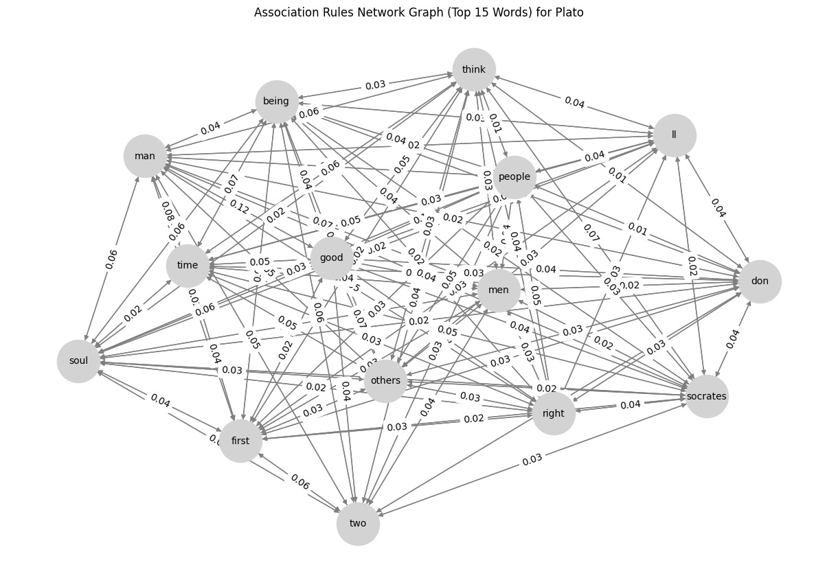
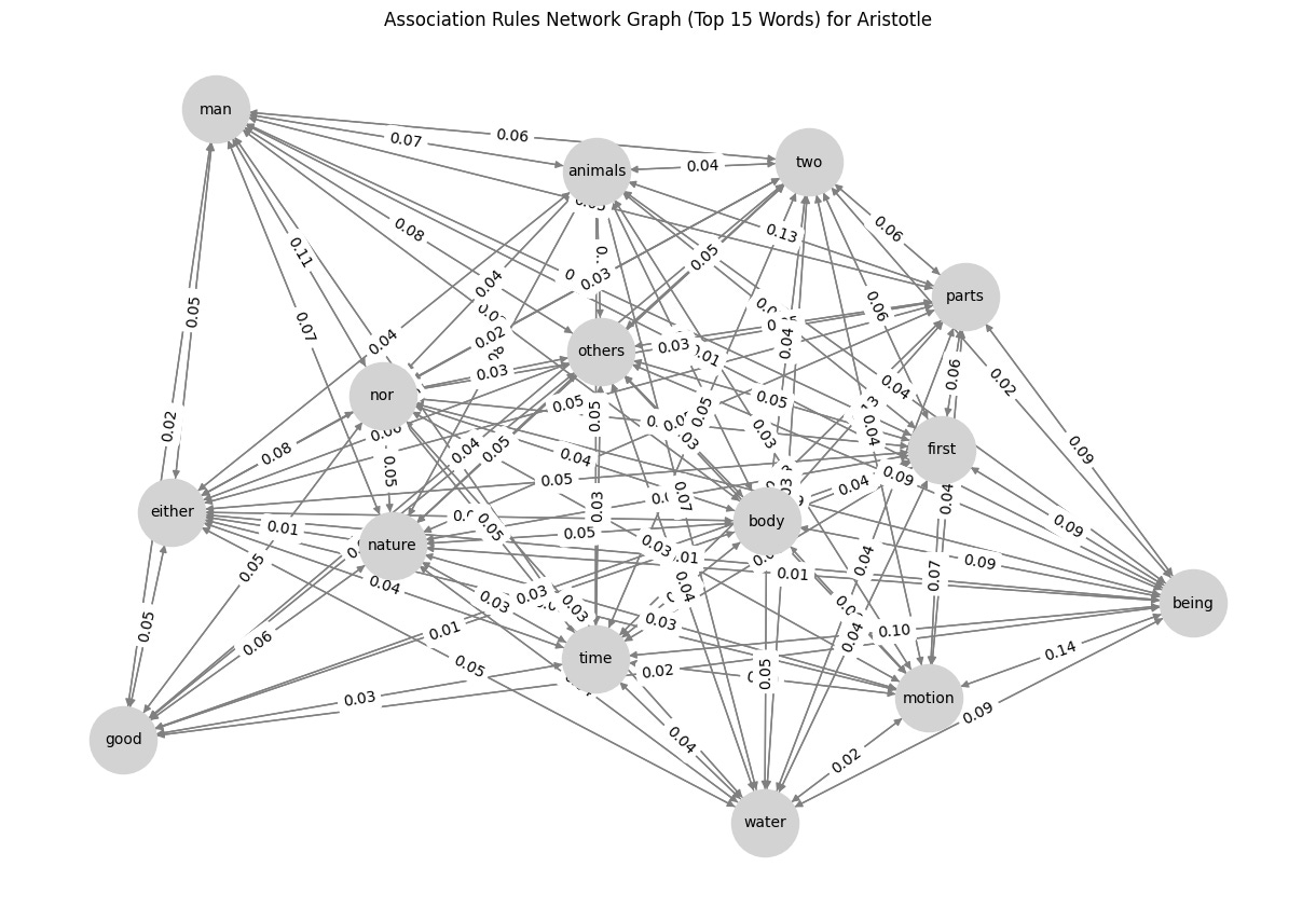
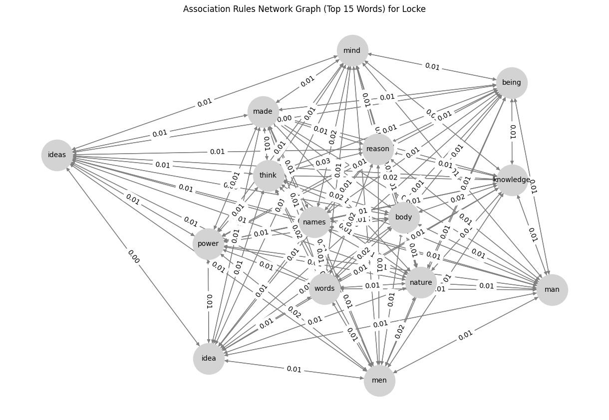
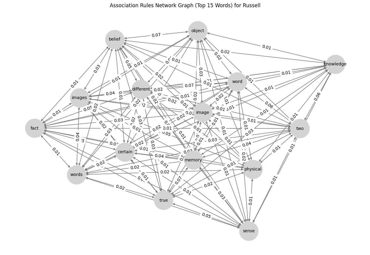
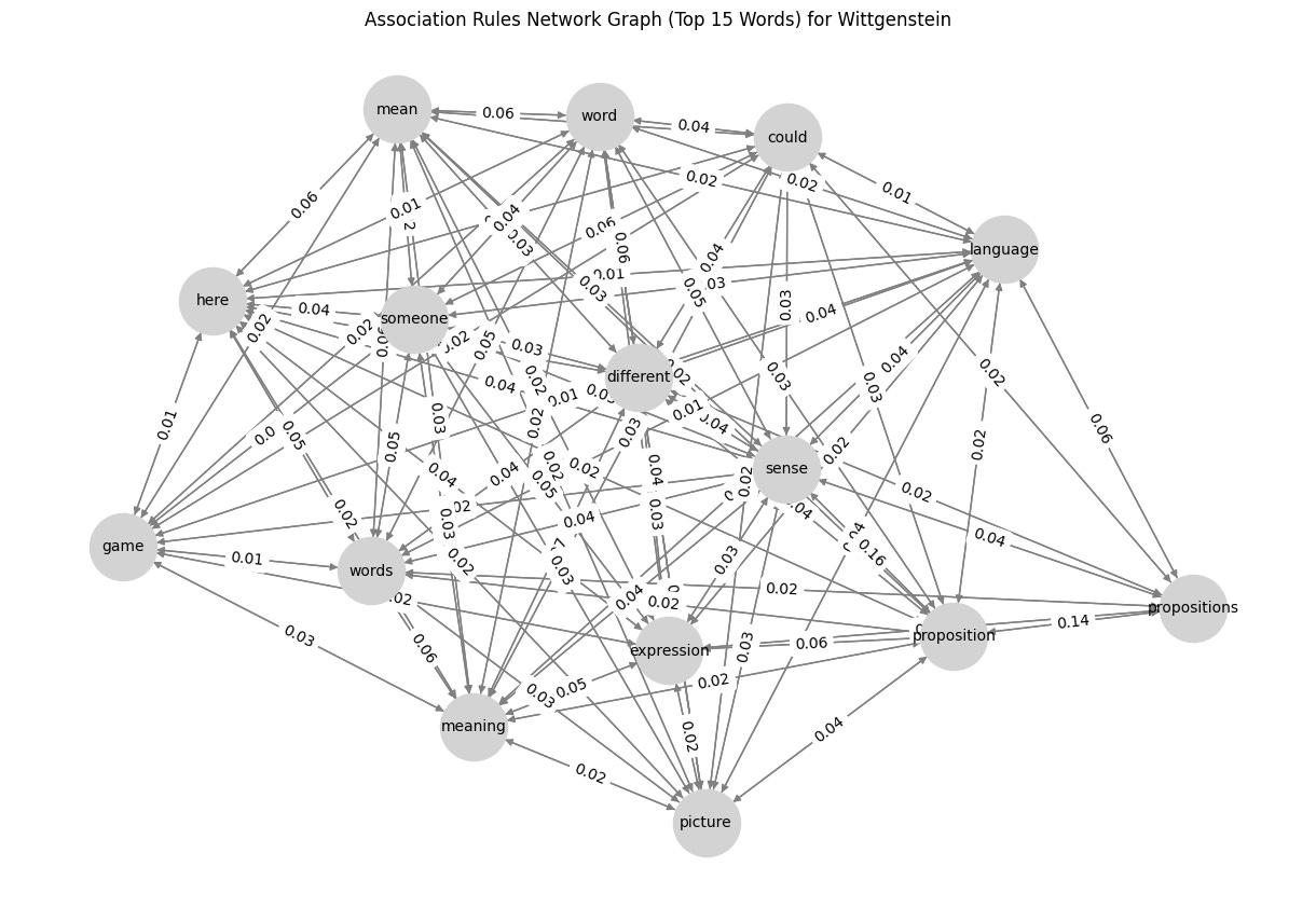
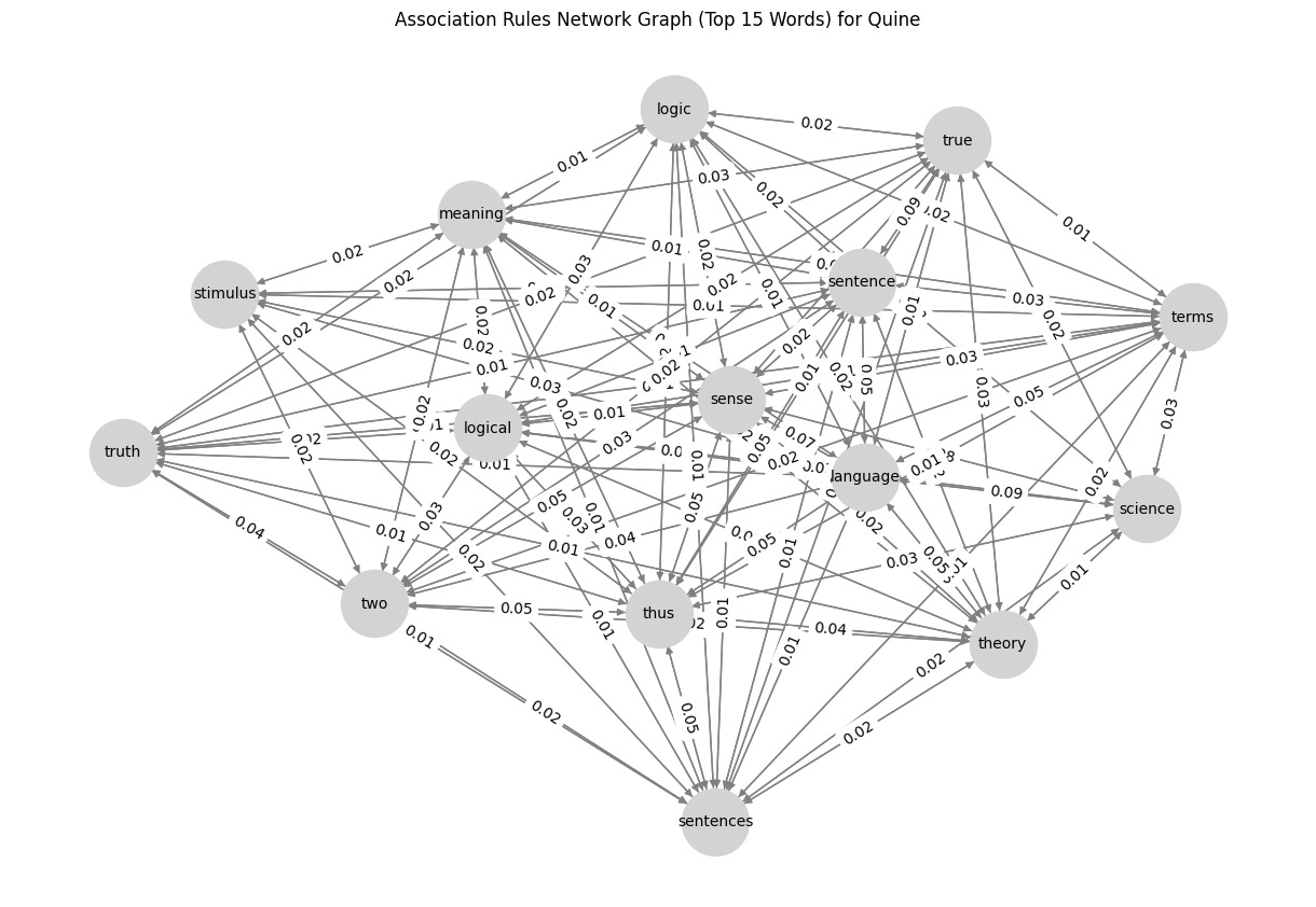
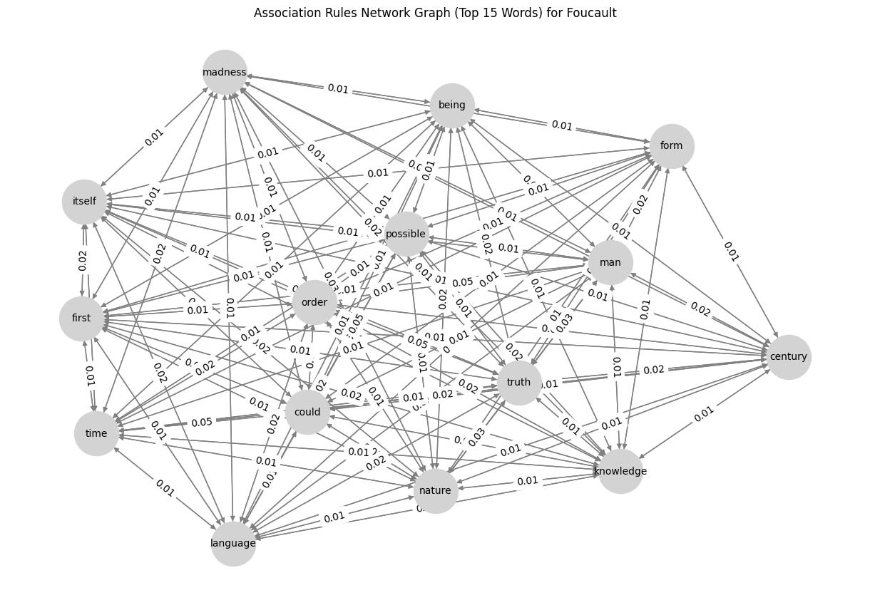
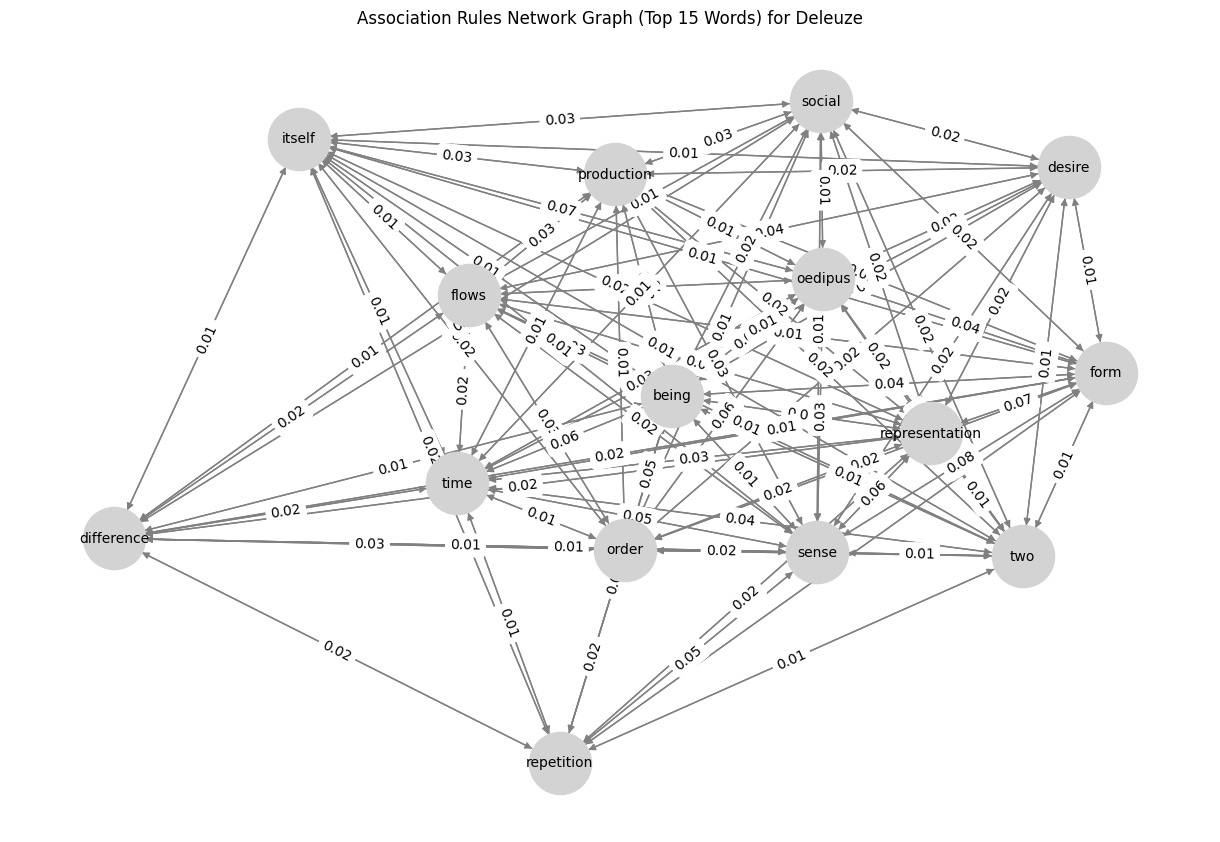
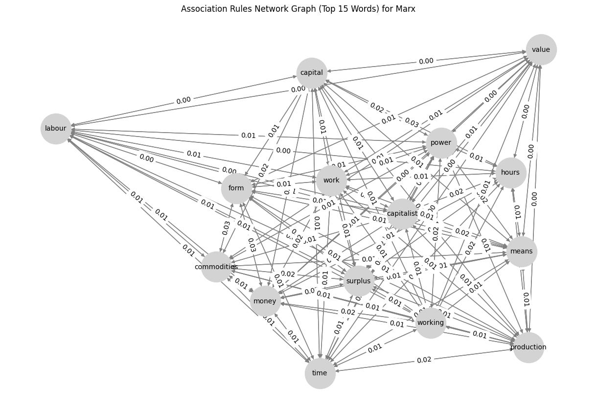
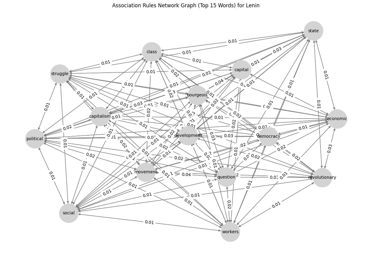
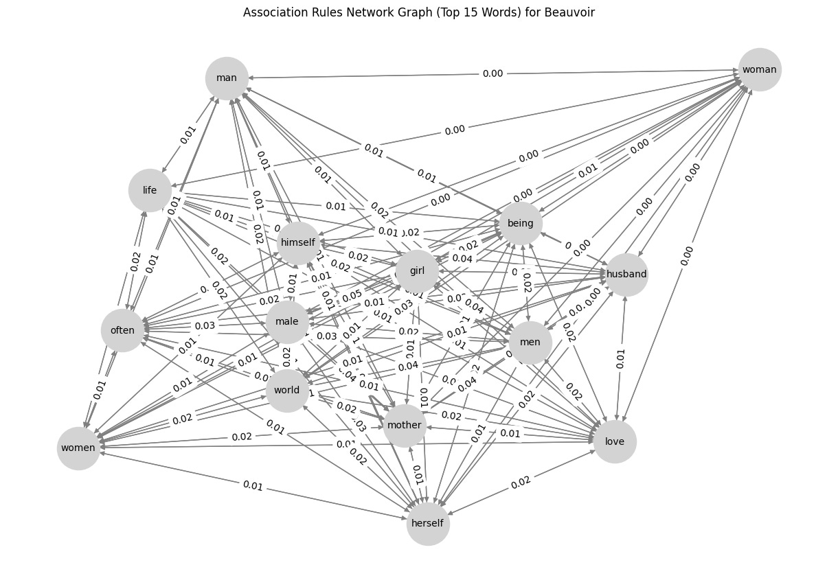
        word_rules_df = pd.DataFrame(word_rules)

Last but not least, constructing a directed graph using NetworkX, where nodes represent words and edges represent association rules. The weight of each edge corresponds to the confidence of the rule, so we can see a visual representation of the strength of associations between words.

G = nx.DiGraph()

        # Add edges to the graph
        for _, row in word_rules_df.iterrows():
            G.add_edge(row['antecedent'], row['consequent'], weight=row['confidence'])

        # Draw graph
        plt.figure(figsize=(12, 8))
        pos = nx.spring_layout(G, seed=42)  # Positioning for nodes
        nx.draw(G, pos, with_labels=True, node_color='lightgray', edge_color='gray', node_size=2000, font_size=10, arrows=True)
        edge_labels = nx.get_edge_attributes(G, 'weight')
        nx.draw_networkx_edge_labels(G, pos, edge_labels={(u, v): f"{d['weight']:.2f}" for u, v, d in G.edges(data=True)})
        plt.title(f"Association Rules Network Graph (Top 15 Words) for {author}")
        plt.show()

So, what’s the result? Check below, and I would like to know what you think about it. Any suggestions for improvements are highly appreciated! 😁